A Color Segmentation Algorithm to Annotate Fine Art Images

演講摘要

目的：

用彩色區域分隔的方法來辨認藝術的畫像，看是一個人物的肖像，還是一個自然風景的畫。

動機：

在網路上可以看到有web museum，也就是網路上的博物館，裡面有很多的畫像、藝術品，有這麼多的畫像要怎麼整理呢？或是要在其中找到一幅畫，但是你不知道作者，只知道畫中有個美女在微笑，那麼只需要打進這樣的想法，這個系統就能幫你找到這幅畫。另外一個動機不是管理美術館，而是管理其他的東西，我們可以用有關影像的資訊來處理、分析這個東西。最後希望達到的功能，是使用者不需要中間去選擇，比如按進哪些字，它就會出現哪本書；在影像方面，我們希望你能夠給它一個範例，它就可以直接幫你找到，你不需要去指導電腦去找到它。

前人的研究：

在資料處理方面，有人提出一個model，主要是想要辨認有肖像在的image，對於portrait image，已經有兩個比較成功的研究。第一個他們是用RGB，我們知道彩色space是RGB，但是我們可以用RGB三個space換成任何一個color space。那麼這個人他是把大的RGB space換成小的rgb的color space。這個人是Miyake在1990年，她能夠把我們皮膚的顏色找出來，因為portrait最多的就人的皮膚的顏色。她發現皮膚的顏色在rg這兩度空間的space上面可以形成一個橢圓形面。第二個發現是有人把RGB換成YES，YES是另外一個color space。這個人是Saber在1996年提出的，他發現有三個族群的顏色，就是皮膚、天空、和草地的顏色在"ES"這個平面上會形成2-D的Gaussian function的分布。

OUTLINE：

首先我們選擇TES的color space，也就是RGB再經過一個matrix的轉換之後成YES。這些係數怎麼來的呢？基本上是經驗的，這些Engineers test很多不同照明程度的圖片，然後來選出這個matrix的係數，她們決定這個叫YES。YES都有它的意義在，Y:事實上就是把一個pixel中RGB的成分所有有關亮度的成分把它拿出來，所以叫liminance。E和S基本上就把它色彩的成分，有顏料的部分取出來。為什麼要選擇這個color space，它的好處是：一、能夠把luminance直接拿出來，譬如同樣一件黑色的襯衫在不同的亮度，它的顏色就會變化。所以很重要的是很容易干擾我們的方法就是它的亮度，所以這個color space它的第一個好處就是能把亮度取出來。第二個好處是可以非常有效率。通常一個圖片都是500x500或是500x1000 ，所以我們要非常有效率來做color space的轉換。因為在這個research當中，因為我們只是需要知道這個pixel的顏料，所以我們只要知道E、S，不需要Y。所以可以發現，E等於是R-G再除以二，所以非常的快速；而S是把R和G加起來，除以二，減掉B，再除以二。所以基本上它的運算非常簡單、直接。第三個好處是它沒有signularities。Sigularities主要是發生在轉換時是nonlinear的matrix，就是剛剛中間那個matrix是nonlinear，就會有singularities的問題出現；但是因為這是一個linear的space，所以沒有這個問題。這就是我們為什麼選擇YES的原因。選擇了這個data之後，就要找mean和covariance的值。因為在這個research是要做人像跟戶外風景，所以選擇兩種種類，一個是皮膚的顏色，另一個是天空的顏色。如果一個2-D的Gaussian function從正上方看過去，它是一個橢圓形。我們可以在網路上找到一些藝術的人像，首先我們要取一些training data，所以我們要截取所有有關於皮膚的顏色的小小的影像，把它轉換成YES的座標。之後，我們就把點畫出來，因為每一個pixel都會有E和S的值，那我們就把它標出個點來。那麼一小張image裡面就會形成一個族群，這樣就可以構成一個像橢圓的圖形，因為我們取的影像不夠多，所以還不是完整的橢圓，跟據統計學的原理，當取的愈多時，統計的分布會趨向一個自然的function。另外是天空的顏色；在畫家的眼裡，天空主要是白色、藍色。但是大家不能只看這二度空間，我們還要看它統計的數目，因為在同一個點上可能有很多點都累積在這裡。所以要將它看成三度空間，它可能是一座山旁邊的一座小山，所以把它按照數目來平均之後，就會產生這兩個橢圓形。接下來就要來教電腦怎麼樣來分辨肖像的人像，還是自然的風景畫。這個方法有六個步驟：

把每個pixel的RGB的值換算成E和S的值。
Histogram的analysis，主要就是lambda的值，因為每一個pixel的值都有E和S的value ，所以可以代入剛才那個橢圓的方程式。然後會算出一個lambda的值。而對於這個lambda的值，可以拿來做統計上的分析，可以找到它非常集中的地方，和不集中的地方。雖然決定了最初的threshold，但是每張圖畫的特性不同，所以這個threshold是可以自己調的。
threshold它會自己移動，跟據我們給它的一個規則，它會開始移動。然後決定一個threshold value叫ta，而一開始的值是tu。
一但決定了這個新的threshold的值之後，把屬於那個族群的全部找出來。
在找出一個族群之後，若它是屬於同一個region的，就可以找出它邊緣的pixel。
linking，就是把每一個邊緣的pixel連起來，那我們就找到了boundary。

跟據這些boundary，我們可以辨別是人物的畫像還是自然的畫像。首先有個digital的color image，輸入電腦把RGB轉換成ES，看有幾種種類，在這裡，我們所用的是皮膚的顏色和天空的顏色。如果要找皮膚顏色，就用剛剛皮膚顏色的mean value和covariance來算出lambda，然後把這些lambda畫成histogram的圖，然後就要開始去找新的threshold value，因為起初決定的是在2，可是它不一定要是2，它會移動。跟據每張畫的特性，我們去找一些可以動的value。我們先找最高點是peaks還有它的峰谷點valleys。我們確定了這點之後，我們就看當初一開始設的initial的threshold是不是在靠近peaks的地方，計算這邊的面積和這個點在下一個valley的面積；看那一個大而往大的方向移動。所以這個地方是一個automatic adaption的algorithm。如果這個不是在很明顯的區域，就選擇原來的值。這個步驟就決定了我們新的threshold的值。用這個threshold的值，可以來決定橢圓形的大小，threshold的值選大一點，橢圓就會變大，反之則變小。而後來分類，若有難區分的地方，就用統計學上的MAP的方法來解決ambiguties。之後選擇edge pixel，把它link，可以找到屬於那一個族群的區域。關於實驗的結果，首先在人像部分，輸入電腦的是蒙娜麗紗的畫像，這張畫像有一個很特別的地方，就是蒙娜麗紗是站在一幅畫像的前面，而那幅畫天空的顏色，很像皮膚的顏色，所以可以看到我們試驗的結果可以發現在人像後面也是很多皮膚顏色的。在我們有一區一區皮膚的區域之後，我們就來找它邊緣的pixel，找出來之後，做了一個大膽的假設，所有人像圖畫的臉，一定在上半部，不可能畫在下半部。人的臉一定會形成一個close loop，而且它的面積會大於整張圖畫的4%。因此我們大膽的假設如果在圖畫的上半部找到一個面積超過4%的封閉區域，就可以辨別這張畫是肖像畫。而另外一個例子是莫內戶外的畫，這張畫是march，有一邊的天空，已被畫家畫的太黑了，不在我們training的範圍，所以我們不去取它。下一步就是找邊緣的pixel，這些pixel是屬於邊邊的pixel。我們又做一個假設，所有的天空會佔一個很大的面積，約佔20%以上，我們找出來是最長的，而且常常是終止在邊緣，不一定是一個open的。若找到一個最長的邊是天空的顏色，就決定就張畫是風景畫。這兩個假設都有缺點，只能做符合的圖。

結論：

這個project有兩個好處，第一個是它全是用自動來辨別的，不用人工去選擇threshold，而自動的去辨別所要的圖。這個algorithm 可以做彩色的分類。之後不同的pixel可以把不同的區間分出來，所用的方法是只要是屬於同一個區域的pixel，它基本上是連續性的，而不會單獨存在，所以pixel會集中在一區。第二個好處是只用到圖畫的彩色，只有在後面步驟才有用到shape，所以用它彩色的部分來分類是非常的簡單。而且計算的時間很短。最後在辨識它是肖像還是自然風景時，有用到面積，所以只用到它的彩色部分和面積部分。

FUTURE WORK：

第一個是可以增加更多的種類，或是keyword。第二個可以加入更多的之前或之後的影像處理，來使得結果更好。如可以把data壓縮，在計算的時間可以縮得很短。第二個region segmentation要做的很準確，目前沒有做simulation的部分，若做simulation的部分，就要重新用個更準確的region segmentation的方法。

演講詳細內容：

今天來講的是有關於彩色影像區域分隔的方法，我個人走的比較靠近影像處理(image processing)還有電腦視覺(computer vision)這方面，這方面還是一個戰國時代；大家都沒有一個最好的方法來解決一個問題，所以就是百家爭鳴，而且沒有人能提出一個讓大家都很服氣的方法。所以今天這個題目也是一樣，這個topic很多人在做，但是沒有人能夠提出最好的方法，只能夠針對某一種特殊用途，來提出她們一個比較好的方法。今天我這個project主要是我在美國修碩士班課的一個project。在project之後，我的教授認為我這個project的idea非常好，所以我把它implement成一個paper，然後在1997台灣開的一個multimedia的conference有發表過。它的topic主要是希望用彩色區域分隔的方法來辨認藝術的畫像，它是一個人物的肖像呢？還是一個自然風景的畫。各位同學如果有任何問題可以隨時打斷我，因為今天這個演講比較重要的是讓大家知道大概一個月的project可以怎麼來做；因為這個東西只花了一個月，所以它有很多需要補強的地方，idea做研究的方式實際上xxxx(聽不清楚)。首先第一個是為什麼要發展這個東西，我的動機是如果妳在網頁上可以看到一些別人已經上網路的叫web museum就是在網路上的博物館，那是非常多非常多的畫像、藝術品，妳怎麼樣來handle它，然後儲存它；甚至妳要找一個畫像，但妳不曉得這幅畫是誰作的，妳只知道這幅畫裡面可以有一個美女在微笑，然後妳就打進這些想法，然後它就可以幫妳找到。另外一個動機是將來不一定是管理一個美術館，而是管理其它東西的時候，所以我們需要一個object-oriented environment。這個環境的特點是有很多資料要處理，第二個現在的處理方式像圖書館的方式是用文字。那麼，我們想要建立一個是用任何有關影像的東西來處理這個environment；所以我們可以用它的color、texture、shape和layout來分析。最後我們要達到的一個用途是使用者不需要中間去選擇，比如按進那些字，它就會出現那本書；在影像方面，我們希望妳能夠給它一個example，它就可以直接幫妳找到，妳不需要去指導電腦去找到它。

基於這兩個動機，我們來看有那些人已經做過這方面的研究。我們分為兩方面，首先在資料處理提出一個model的人，主要她們是想要辨認有肖像在的image；所謂肖像的image就是有個人，像各位的大頭照一樣。那它是一個portrait image的話，有兩個比較成功的work已經有了。第一個她們是用RGB，我們知道彩色space是RGB，但是我們可以用RGB三個space換成任何一個color space。那麼這個人她是把大的RGB space換成小的rgb的color space。這個人是Miyake在1990年，她是能夠把我們皮膚的顏色，因為portrait最多的就人的皮膚的顏色。她發現皮膚的顏色在rg這兩度空間的space上面可以形成一個橢圓形的group裡面。

第二個發現是有人把RGB換成YES，YES是另外一個color space。這個人是Saber在1996年提出的，她發現有三個族群的顏色，就是皮膚、天空、和草地的顏色在"ES"這個平面上會形成2-D的Gaussian function的分布。這篇paper其實就是這個人paper的延伸。我們希望用她的model來做更多的事情，最後達到區域分隔的效果。在object-oriented environment方面，已經做過的有很多，這個大家都有聽過。像IBM它有發展一個軟體叫做Query-by-Image-Content，譬如說，妳要找一個紅白相間的T-shirt的圖案，妳只要把這個圖案放在user choice這邊，它就會找出在它database中所有有紅白相間的圖案都給妳；在1993年已經commercial。MIT有一個photobook在1993年。ETL在1991年有個處理art museum的軟体。University of Miohigan 在1993年也做出一個軟体叫做Xenemania在1993年，最近的是1995年由Columbla Univ.出了一個Multimedia testbed。

進入今天talk的outline，首先我們今天要介紹的是第一個我們怎樣去選擇一個color space，然後選擇一個data modeling。第二個要介紹的是我用的方法最後來解決利用彩色區域分隔的方式。這個方法有三個步驟；第一個步驟是因為在一個iamge裡面，每個單位就是pixel，第一個是用pixel來分類；就是那個pixel 它是屬於什麼顏色，我們就把那個pixel 分為那一類。在妳把所有同個顏色，譬如說人的肖像來講，臉的方面如果能夠可以把所有皮膚的顏色pixel都找出來，之後，我們就把pixel整合起來，變成一個區域，然後把它分隔出來之後，最後我們希望把它的boundary能夠決定。我這篇給大家看的是一個應用，怎樣讓電腦自動地分辨一個美術的圖畫是人的肖像還是自然景觀的圖畫。最後會給大家看一些實驗的結果。

首先，我們就來選擇一個color space；這個color space叫YES，這個YES是由一個日本的學會，叫做Motion Picture and Television Engineers的學會所提出來的，也就是RGB再經過一個matrix的轉換之後，它會轉換成YES。這些係數怎麼來的呢？基本上是經驗的，這些Engineers test很多不同照明程度的圖片，然後來選出這個matrix的係數，她們決定這個叫YES。YES都有它的意義在，Y:事實上就是把一個pixel中RGB的成分所有有關亮度的成分把它拿出來，所以叫liminance。E和S基本上就把它色彩的成分，有顏料的部分取出來。

我為什麼要選擇這個color space，如果大家有興趣可以看看image processing的book，它會寫說color space就一個大table有很多人提出不同的用途。這個是比較新的題材，所以妳的教科書找不到。它的好處是：一、能夠把luminance 直接拿出來，譬如同樣一件黑色的襯衫在不同的亮度，它的顏色就會變化。所以很重要的是很容易干擾我們的方法就是它的亮度，所以這個color space它的第一個好處就是能把亮度取出來。

第二個好處是可以非常有效率。因為通常一個圖片都是500x500或是500x1000 ，所以我們要非常有效率來做color space的轉換。因為在這個research當中，我們只需要E和S，我們不需要Y，因為我們只是需要知道這個pixel的顏料，所以我們只要知道E、S。所以可以發現，E等於是R-G再除以二，所以非常的快速；而S是把R和G加起來，除以二，減掉B，再除以二。所以基本上它的運算非常簡單、直接。

第三個好處是它沒有signularities。Sigularities主要是發生在轉換時是nonlinear的natrix，就是剛剛中間那個matrix是nonlinear，就會有singularities的問題出現；但是因為這是一個linear的space，所以沒有這個問題。所以這就是我們為什麼選擇YES的原因。

第二個我們要選擇怎樣來model這個data；我選擇了Saber的方法，因為她的modeling的本質、feture是很合適的，我自己有check過，所以我選擇她的方法。所謂的2-D Gaussian probability density function這就是一個它標準的一個probability function，大家可以看到，是這樣子。然後這邊有個exponential，然後我們發現這邊，這個是mean vector然後k是covariance matrix，然後這邊首先x是代表每一個pixel的e值和s值。mean value是e那個軸的mean value和s軸的mean value；covariance就是e和s的相關係數。我們可以發現，如果我們把exponential上面的係數是決定這個Gaussian function是比較胖還是比較瘦。那這個coefficient是決定這個Gaussian function的高度，最高的那個點在那裡。因為Gaussian function 在三度空間從正上方看過去，它是一個橢圓形。那上面這個coefficient是決定這個橢圓的公式。如果我們把這個equaltion算出一個值，我們訂它叫lambda，將來用做自動的algorithm的primate(不清楚)。

我們選擇了這個data之後，這個mean和covariance的值怎麼找，接下來，就要跟大家講，因為這個東西以後如果妳們有興趣做data方面的都會用到。因為在這個research我是要做人像跟戶外風景，所以我選擇兩種種類，一個是皮膚的顏色，另一個是天空的顏色。如果一個2-D的Gaussian function從正上方看過去，它是一個橢圓形。這就是我training data所產生的資料。star所形成的是皮膚所成的族群，而圈圈所形成的是天空形成的族群。我們要怎麼做呢？首先，現在網路非常的發達，可以在網路上找到一些藝術的人像。以下是大家看到很熟悉的面孔--梵谷。首先我們要取一些training data ，所以我們要截取所有有關於皮膚的顏色的小小的影像，把它轉換成YES的座標。之後，我們就把點畫出來，因為每一個pixel都會有E和S的值，那我們就把它標出個點來。那麼一小張image裡面就會形成一個族群。我選了十個人像的畫，就可以構成這個。妳看它看起不像橢圓，因為我們取的影像不夠多，跟據統計學的原理，當取的愈多時，統計的分布會趨向一個自然的function，所以這個原因是我們取的不夠多。

另外，這個圖是天空的顏色；在畫家的眼裡，天空很多都是有雲的顏色，所以主要是白色、藍色；這個奇怪的族群是有一張畫，它天空的顏色非常的藍。所以會造成這兩個族群分開。但是大家不能只看這二度空間，我們還要看它統計的數目，因為在同一個點上可能有很多點都累積在這裡。所以要將它看成三度空間，它可能是一座山旁邊的一座小山，所以把它按照數目來平均之後，就會產生這兩個橢圓形。

找到這個之後，就可以決定，這兩個點，就是族群的中心。而橢圓形的大小，是要由自己去決定；如果這個橢圓形在三度空間看起來很胖，那麼這個橢圓就要取大一點；如果是一個很纖細的橢圓，就要找瘦一點。所以這要去看一下三度空間的分布。最後會得到它的平均值，就是剛才那些橢圓的中心位置，然後跟它的大小，還有location的方向可以決定covariance。橢圓的大小，要決定多大是非常conferdant(不清楚)的inteval。也就是說，我確定所有的點在這個橢圓之內都是這個顏色。所以，跟據我個人所用的training data，我決定兩個都是2，那只是湊巧，不一定要一樣。

決定了color space和data modeling的方式之後，這裡show一下我用的其它的training data，在人像方面，我用的有達文西、雷諾爾、梵谷的；所以它們的顏色是差別很多的。而在室外的自然景觀，我所用的是這些，像這個天空就非常的藍，和海水一樣，這就是剛才脫離主要族群的部分。有的天空充滿了雲，還有的天空是泛紅。

在自然景觀方面，我所著重的畫家是莫內。基本上大家可以有個idea就是將來可以用來處理照片，為什麼我這個project 是做美術的畫，是因為老師規定所有的project都要和美術有關，所以大家不可以用照片。

接下來，就要來教電腦怎麼樣來分辨肖像的人像，還是自然的風景畫。這個方法有六個步驟，第一個步驟就是把每個pixel的RGB的值換算成E和S的值，我們不需要它的亮度。第二個步驟就是Histogram的analysis，主要就是lambda的值，因為每一個pixel的值都有E和S的value ，所以可以代入剛才那個橢圓的方程式。然後會算出一個lambda的值。而對於這個lambda的值，可以拿來做統計上的分析，可以找到它非常集中的地方，和不集中的地方。雖然決定了最初的threshold，但是每張圖畫的特性不同，所以這個threshold是可以自己調的。所以下一個步驟就是threshold 它會自己移動，跟據我們給它的一個規則，它會開始移動。然後決定一個threshold value叫ta，而一開始的值是tu。下一個步驟是一但決定了這個新的threshold的值之後，把屬於那個族群的全部收集、找出來。下一個步驟是在找出一個族群之後，若它是屬於同一個region的，就可以找出它邊緣的pixel，下一個步驟是linking，就是把每一個邊緣的pixel連起來，那我們就找到了boundary。跟據這些boundary，我們可以辨別是人物的畫像還是自然的畫像。

首先有個digital的color image，輸入電腦，電腦就把RGB轉換成ES，看有幾種種類，在這篇paper 中，我們所用的是皮膚的顏色和天空的顏色。如果要找皮膚顏色，就用剛剛皮膚顏色的mean value和covariance來算出lambda，算出lambda之後，就把這些lambda畫成histogram的圖，這圖看起來，就是像這樣子。算出了所有的值，然後畫出這個histogram，就要開始去找新的threshold value，因為起初決定的是在2，可是它不一定要是2 ，所以它會移動。跟據每張畫的特性，我們去找一些可以動的value。我們先找最高點是peaks還有它的峰谷點valleys。我們確定了這點之後，我們就看當初一開始設的initial的threshold是不是在靠近peaks的地方，我們會計算這邊的面積和這個點在下一個valley的面積；看那一個大而往大的方向移動。所以這個地方是一個automatic adaption的algorithm。如果這個不是在很明顯的區域，就選擇原來的值。這個步驟就決定了我們新的threshold的值。

用這個threshold的值，可以來決定橢圓形的大小，因為改變了這個threshold的值，橢圓就會變化。threshold的值選大一點，橢圓就會變大，反之則變小。而後來分類，若有難區分的地方，就用統計學上的MAP的方法來解決ambiguties。之後選擇edge pixel，把它link，可以找到屬於那一個族群的區域。

現在我們來看一下實驗的結果，首先在人像部分，輸入電腦的是蒙娜麗紗的畫像，這張畫像有一個很特別的地方，就是蒙娜麗紗是站在一幅畫像的前面，而那幅畫天空的顏色，很像皮膚的顏色，所以可以看到我們試驗的結果可以發現在人像後面也是很多皮膚顏色的。在我們有一區一區皮膚的區域之後，我們就來找它邊緣的pixel，找出來之後，做了一個大膽的假設，所有人像圖畫的臉，一定在上半部，不可能畫在下半部。人的臉一定會形成一個close loop，而且它的面積會大於整張圖畫的4%。會去找畫上可以連成的區域，而且這個區域的面積是大於4%的。因此我們大膽的假設如果在圖畫的上半部找到一個面積超過4%的封閉區域，就可以辨別這張畫是肖像的畫。而另外一個例子是莫內戶外的畫，這張畫是march，有一邊的天空，已被畫家畫的太黑了，不在我們training的範圍，所以我們不去取它。下一步就是找邊緣的pixel，這些pixel是屬於邊邊的pixel。我們又做一個假設，所有的天空會佔一個很大的面積，約佔20%以上，我們找出來是最長的，而且常常是終止在邊緣，不一定是一個open的。若找到一個最長的邊是天空的顏色，就決定就張畫是風景畫。這兩個假設都有缺點，只能做符合的圖。

結論如下，第一個好處是它全是用自動來辨別的，不用人工去選擇threshold，而自動的去辨別所要的圖。經由pre-specified的keyword。這個algorithm 可以做彩色的分類，首先可以將pixel分成想要的種類，而且計算非常的簡單。之後可以把不同的pixel可以把不同的區間分出來，所用的方法是只要是屬於同一個區域的pixel，它基本上是連續性的，而不會單獨存在，所以pixel會集中在一區。第二個是只用到圖畫的彩色，只有在後面步驟才有用到shape，所以用它彩色的部分來分類是非常的簡單。而且計算的時間很短。最後在辨識它是肖像還是自然風景時，有用到面積，但是shape還沒有用到，所以只用到它的彩色部分，還有面積部分。

這個project 未來還有很多可以做，第一個是可以增加更多的種類，或是keyword。第二個可以加入更多的之前或之後的影像處理，來使得結果更好。如可以把data壓縮，因為圖的pixel都很多，如果可以把1000x1000變成500x500，在計算的時間可以縮得很短。第二個region segmentation要做的很準確，目前沒有做simulation的部分，若做simulation的部分，就要重新用個更準確的region segmentation的方法。

待會會show一些目前在做的research，也是關於segmentation，區域分隔的東西，但是是用在黑白影像方面，而且是用在親子dna鑑定的圖像上面。

在dna上面，我們所發展的是自動數出有多少條dna的lane，在band上面，我們要作的是數出每條lane上面有多少條band，在spot方面，要自動地數出有多少個斑點。現在把圖片秀給大家看，因為誠如我剛才所說的，所有的方法都是商業機密，不能直接告訴大家。

這張圖畫就是所謂的dna的band，這可能是你爸爸的dna，如果你是你爸爸的小孩的話，那麼你一定要是你爸爸跟你媽媽的聯集。所以如果你出來有你爸媽沒有的，那麼你就不是你爸媽的小孩。現在為甚麼dna檢測的時間要那麼慢的原因就是，第一個要跑出這張圖片就要花上半天的時間，因為它放在像果凍上面的東西，要在果凍上挖隧道，把dna放進這些隧道裏面，然後再放進電解池，然後dna就會根據它的分子量的重量跑，跑出來會分布不同的形狀，再分析彼此之間的關係，最重要就是算出這些分子量。所以我們影像處理的人要幫助他們從這些位置來決定分子量，因為越重的跑的越慢。

第一張圖片進來後，我們大概只花半秒鐘就可以知道這些所有band的位置還有它有多少的lane，所以電腦馬上告訴你它有8個lane，32個band，用c++來implement的。如果有人喜歡的話，就是把每個band框起來，或者是把每個band的邊緣都找出來，來算band所佔的面積，這只是顯示方式的不同。

第二個example就複雜的多，它有好幾個channel，所以這跑出來有20條，中間一條是空的。所以這也大概花一秒鐘就可以找出它有19個lane，77個band。

第三個demo的影像就是有時候channel挖得歪了，或者電解池的電位不是對得很準，所以會往兩邊跑。這個比較大，所以花了3秒鐘找出來它有10條lane有146個band。

在dna看完之後，這個是不同的病菌，像腸病毒太小，我們大概是找一些細菌，像大腸桿菌。你可以發現這是黑白影像，它有黑色的點和白色的點。而且很困難的，因為黑色的點光線一照會反光。所以電腦要數出白色的比較容易，黑色的比較難。這個大概也是一秒鐘，可以數出它有13個白點。比較挑戰性的是當兩個白點非常靠近的時候，而且一大一小，怎麼樣分出來。然後黑色點連在一起的時候，它要怎麼數出來，所以數出來有16個黑點。

跟大家透露一點商業機密，因為我們的客戶都知道，但是你們比較聰明，或許聽了就會作。

在dna方面，我們所用到的是一度空間的peak detection，就是找它的peak。把每個band在三度空間給model一個小山峰，然後再用traversal linking，依pixel連起來。那麼在spot上面，是二度空間的peak detection，如果你們把影像的長度看成三度空間的話，就是2-dimension of peak detection，一樣把邊緣連起來。黑色的點就tricky一點，因為要考慮到黑色照到燈光會反光。

在剛剛講的彩色方面，我的公司也即將發展一些彩色處理的儀器。首先要如何加強彩色影像，因為彩色影像都有noise。所以左邊有noise的影像經過處理以後，所有的斑點全部不見了。

再秀一個分類例子，譬如說有三種細胞或三種不同病毒的顏色。像我們要藍色的細胞而已，我們就找藍色的。用剛剛教給大家的方式，找到它的邊緣，就可以計算出每一藍色細胞的特性：它的面積，多圓，最大跟最小值，就是裏面的pixel value。

所以這邊結束我今天跟大家作的presentation，希望大家會喜歡，謝謝大家！

q:橢圓不會有交集嗎?
a:如果有交集時，就要用統計學的一個方法，有一點在兩個橢圓交集的地方；事實上，這個橢圓的大小也是由妳來決定。要按照資料的特性來選擇橢圓的大小。這只是某個區間，因為Gaussian function 還會繼續至兩個一定會有交集的地方。在交集的地方，就把pixel拿出來，看它比較靠近那一個橢圓，就是那一個的族群。

q:這樣判辨就會有錯誤了?
a:當然會有error，當妳非常confuse時，所以可以不要選擇那個pixel，通常ambiguous的pixel 是在比較discrete的地方，因為我們要找的是一個region，所以可以不要它。

q:對於照片，也是一樣嗎?
a:也是要去找很多照片來training，來把它轉換成E和S，後找出它的族群出來。

q:那照片不是會比較xx(不清楚)，因為畫家的???
a:對，今天我所展現的係數，它是不能用在nature的影像方面。它只是在係數的差別，但方法是可以應用在照片的。若以後自己要做，原來作者Saber 是做在照片上皮膚的顏色，可是Saber 這個人可能有種族歧視，她只做白人的皮膚，所以她的test images全部都是白人。所以要自己做的就是這個部分。會得到不同區域的橢圓形。但是原理是一樣的。而且當兩個橢圓靠近的時候，就要用統計學上，看那一個probability比較大，來決定它是屬於那一個族類。

q:剛才有說到Columbla Univ.的有做一些沒有種族歧視的，後來發現各個人種都有一些各自共同的係數。
a:基本上膚色跟照明很有關係，所以有些人皮膚很黑，強光一打還是會變得很白。像婚紗照，有些人很黑，可是看起來卻很白，就是因為照明的關係。所以我覺得顏料有它的本質，所以YES 這個color space是大家可以考慮的一個space。可是它不是唯一的。所以現在有很多的engineers還在找適合她們應用的color scaoe。我今天只是提出一個idea而已。

q:不同畫家的畫風，可不可以由設定出來的係數看出來?
a:可以，像達文西畫的美女都很蒼白，而雷諾爾畫的就比較健康。會形成不同的族群，但是會很靠近，因為基本上，都是皮膚的顏色。所以在皮膚方面比較難分辨，但稍微可以看出來。像天空方面，如果是藍藍的，像那種青色的天空，它就特別的脫離白色的區域。因為大部分的天空，雲都很多，所以會比較靠近白色的區域。經由投影和原來的顏色不一樣，所以這是轉換過程中的一個distortion。

q:錯誤率上，有多少?
a:目前只有兩個test，所以沒有辦法很有效的測出，但是這個algorithm在後面假設有很大的漏洞，如若是兩個人臉的肖像，那面積就可能會減少，所以必須做更多的考量。如果皮膚顏色和天空顏色，沒有超出我訓練的影像的範圍之外，就可以分辨的出。但是畫家會常用不同顏色來表現，如畢卡索就有一張紫色的臉，那就完全測不出來。所以在顏色方面是蠻robust，可是如果更多的人，或是顏色的變動，就沒有辦法了。

相關資料

Introduction

In text, There are some important topics that have been introducted and we don't repeat it again. But some topics that don't introducte may make some mistake if somebody never learn about video or multimedia. We will talk about it's detail and where we find them out in the world wide web. Just as the speaking that there some topics and technicality but that don't touch it detial and what we will introduce are four topics - Color space, RGB, CMYK and Region-based segentation - There are also some relative topcs such as Query-by-Image-Content that can find out the digital image form your query.

Colorspace

1.what is colorspace

Color Space Definitions

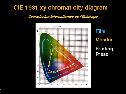
Chromaticity Diagrams

The CIE 1931 xy

This color space is a mathematical representation of the human eye's response to color. Note that this color space is non-linear! It's a 3-D model that is "unfolded" like a Mecador projection map of the earth.

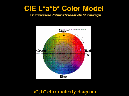
CIELAB

LAB color is the same model revised to be a linear color space. This model works best to define color on a computer because of its linear nature. A and B define the hue and saturation of the color where the L value or "Luminance" comprises the Z axis through the middle. The 0,0 point of the diagram is the "white reference" and defined as the color temperature. With the xyY defination of LAB (See "Printing Inks Setup" in Photoshop), the Y value can be calculated through a simple equation.

2.RGB

Exact color reproduction is and has always been the goal that is difficult to achieve 。Many applications use the Intenational de l’Eclairage’s CIE XYZ color model (or color space) as a basis to prepare a color rendering before it is output to a device。The CIE XYZ color model provides a mathematical representation of all visible colors and is hardware-device-independent。However，even a device-independent color model does not work well in practice for following reasons:

The color range of the printer and the display do not match since monitors use the RGB color model and printer use the CMYK color model，the printer driver make the best suited for monitors since screen phosphors generate color by additive mixing。On the other hand ，the CMYK color model is best suited for printers since cyan ，magenta ，yellow ，and black use subtractie mixing to create colors on paper。
The color ranger of a device varies with the technology as each technology has its own color range 。
Even after the devices are calibrated，the colors vary when printed。

So what is the solution ? The monitor screen colors are output to a printer consistenty ; that is ，the application outputs the same color every time a paticular color is used。The devices are regularly calibrated to ensure that the color rendering of the printer matches the screen output。

3.CMYK

Introduction one CMYK publishes the very best work from students in advertising, design, illustration and photography. As judged by leaders in each field.CMYK is then sent to individual creative directors, art directors and principals at over 15,000 advertising agencies and design firms across the U.S. and abroad. Along with agency and design firm features, top student and school profiles , hints and tips from the pros, and much more, CMYK allows creative leaders the opportunity to see who's hot, and who to hire – and gives students the chance to see what their competition is up to. With a total circulation of 30,000, CMYK is also used as the curriculum at the nation's art schools and universities, and can be found in leading book chains throughout the U.S., Canada, Japan and Sweden at Barnes and Noble, Borders, Crown Books, Tower Books and Keplers.
Introduction two CMYK offers Scitex imagesetting for superior film output. Our Scitex system includes 2 fully equipped workstations and a large format Dolev 800 imagesetter for plotting films up to 32"x44". We also have an AGFA 7000 imagesetter for films up to 22"x26". We can provide you with positives or negatives at any line screen up to 625 lpi. Custom screens ara available, including Scitex FULLtone stochastic screening. For screenprinters, we offer custom screen angles and line screens as at 55 lpi or lower.We offer trapping with Scitex Full Auto Frames to provide automatic RIP trapping of your entire desktop lie on our Scitex workstations.

Save money by stripping your files electronically! We can provide paginations for QuarkXpress and Pagemaker files. We offer the QuarkXpress Xtension InPosition for printer spreads, 4-up's and 8-up's, or we can provide manual impositions.

4.Relation

The Commission International L'Eclairage (CIE) diagram of color space shows the range of visible color and the much smaller gamut ranges of RGB and YMCK color space. This is a 2-dimensional representation of something that is better described by a 3-dimensional model. The concept of three dimensions of color spaces was first articulated by Albert Munsell in 1914. Munsell defined even visual steps of color in hue, value (saturation), and chroma (equivalent grayness). Other early work in describing three-dimensional color space was contributed by Ostwald, who conceived that pure color hues should be lightened by adding white and darkened by adding black. His 3-D model took the shape of two equal cones joined at the base. In 4-color process, less dot density allows more light to be reflected from white paper, and colors are darkened by adding black, which is neutral and does not affect cast.

In 1931, the CIE refined the mathematical notation system for the three dimensions of color space by adding the concept of a standard observer with standard illumination. As the electronic pre-press industry seeks desirable standardization, a consensus formed using CIElab notation values (with 1,a,b being the coordinates for hue, saturation, and brightness, the evolutionary way of describing the three dimensions of color space originally detailed by Munsell). In the patented TRUMATCH approach to 4-color process, lighter values of a hue are achieved by reducing dot density and allowing more "white" paper to show through; darker colors are achieved achromatically by adding black. TRUMATCH affords the graphic designer a proportionately gradated color palette through the ability to select YMCK output values to 1% targets using desktop software and imagers. The CIE diagram illustrates the range of visible color space. Notice that RGB space and YMCK space are not congruent. Many RGB colors are not reproducible in YMCK space, and the reverse is also true. Furthermore, many solid-ink swatches fall beyond both gamut ranges. Publishing in 4-color process with the TRUMATCH Colorfinder for color selection will give an achievable palette of over 2,000 colors, blanketing the YMCK gamut range in smooth, proportionate steps.

Color space http://www.barco-usa.com/colorspa.htm

CMYK

Relation http://www.trumatch.com/articles/anchor.htm

Region Segmentation

General Approach

There are two classes of techniques for color indexing: indexing by (1) global color distribution and (2) local or region color. An important distinction between these techniques is that indexing by global distribution enables only whole images to be compared while regional indexing enables matching between localized regions within images. Both techniques are very useful for retrieval of images and videos but are suited for different types of queries.

Color indexing by global distribution is most useful when user provides a sample image for the query. For example, if the user is interested in finding panoramic shots of a football game between two teams, then by providing one sample of the image others can be found that match the query image. Color indexing by global color distribution works well in this case because the user is not concerned with the positions of colored objects or regions in the images. However, when the user is interested in finding things within images the global color distribution does not provide the means for resolving the spatially localized color regions from the global distribution.

On the other hand, color indexing by localized or regional color provides for partial or sub-image matching between images. For example, if the user is interested in finding all images of sunsets where the sun is setting in the upper left part of the image, then regional indexing enables this query to be answered. Localized or regional color indexing is generally more difficult because it requires the effective extraction and representation of local regions. In both cases a system is needed for the automated extraction and efficient representation of color so that the query system provides for effective image and video retrieval. In this paper we present a technique that applies to both global and localized color region extraction and indexing.

The feature extraction system consists of two stages: (1) extraction of regions and (2) extraction of region properties as shown in Figure 1. An automated system performs both stages without human assistance. It is typically stage 1 that is either manual or semi-automatic when the system is not fully automated. The representation of region color is often more robust when the region extraction is not automated.

Figure 1: General approach for color image feature extraction.

Region Extraction/Segmentation

The goal of the region extraction system is to obtain the spatial boundaries of the regions that will be of most interest to the user. The process of region extraction differs from image segmentation. Segmentation corresponds to a complete partitioning of the image such that each image point is assigned to one segment. With region extraction an image point may be assigned to many regions or to none. Conceptually, this is more desirable than segmentation because it supports an object-oriented representation of image content. For example, an image point corresponding to the wheel of a car can simultaneously belong to the two different regions that encapsulate respectively the wheel and the car as a whole.

There are several techniques for region extraction. The least complex method involves (1) manual or semi-automated extraction. In this process the images are evaluated by people and the pertinent information is confirmed or identified visually. This is extremely tedious and time-consuming for large image and video databases. Another procedure for region extraction utilizes a (2) fixed block segmentation of the images. By representing color content of small blocks independently there is greater likelihood that matches between regions can be obtained. However, it is difficult to pick the scale at which images should be best blocked. A third technique involves (3) color segmentation. There have been several techniques recently proposed for this such as color pairs [CLP94] and foreground object color extraction tools [HCP95].

We propose a new technique which partly employs the color histogram (4) back-projection developed by Swain and Ballard for matching images [SB91][SC95]. The basic idea behind the back-projection algorithm is that the most likely location of a spatially localized color histogram within an image is found by the back-projection onto the image of the quotient of the query histogram and the image histogram. More specifically, given query histogram g[m] and image histogram h[m], let . Then replace each point in the image by the corresponding confidence score B[m,n] = s[I[m,n]]. After convolving B[m, n] with a blurring mask, the location of the peak value corresponds to the most likely location of the model histogram within the image. In small image retrieval applications this computation is performed at the time of query to find objects within images [SB91][EM95]. However, for a large collection it is not feasible to compute the back-projection on the fly. A faster color indexing method is needed.

We extend the back-projection to the retrieval from large databases by precomputing for all images in the database the back-projections with predefined color sets. By processing these back-projections ahead of time, the system returns the best matches directly and without new computation at the time of the query. More specifically, we modify the back-projection algorithm so that it back-projects binary color sets onto the images. Instead of blurring the back-projected images we use morphological filtering to identify the color regions. This process is described in greater detail in later sections.

Region Feature Extraction

Once the image regions are identified, each region is characterized and represented using a feature set. The goal of color representation is to accurately capture the salient color characteristics of the region in a low-dimensional vector. Two choices for simple color features are (1) mean color and (2) dominant color of the region. They both use only a 3-D vector to represent the color of the region. The comparison measurement is fairly easy to compute but the discrimination is inadequate. An alternative is to use (3) color histograms. A color histogram is a high-dimensional feature vector typically having greater than 100 dimensions and the comparison of histograms is computationally intensive. They are best suited for representation of global color rather than local color regions because of storage requirements and the large number of computations required at query time.

We propose a new approach for representation of color content which is well matched to the binary color set back-projection region extraction. We represent region color using a (4) binary color set that selects only those colors which are sufficiently present in the region. Since the color sets are binary vectors, they can be indexed efficiently, i.e., using a binary tree, rather than requiring substantial computations to compare histograms at query time. The binary set representation of color regions and indexing is described in detail in the following sections.

Color Image Retrieval Systems

Recently, several systems have appeared for the content-based retrieval of images. The QBIC system [FFN93] provides for the retrieval of images by color, texture and shape. It supports two classes of color content - global and local. In the QBIC system the extraction of local regions is handled manually by requiring a person to draw region boundaries using a mouse. Both the global and local color information is represented by mean color and color histogram. The QBIC system also uses a quadratic distance metric for comparing histograms. Because the quadratic distance measure is very computationally intensive, the mean color distance is used as a pre-filter for color queries [HSE95].

VisualSEEk

We are currently developing VisualSEEk: a content-based image/video retrieval system for the World Wide Web. VisualSEEk supports query by color and texture and spatial-layout. Other features such as shape, motion and embedded text will be incorporated in the near future. The system (see Figure 2) provides the user with a highly functional and platform independent Java user-interface which collects the user's query. The query is communicated to the VisualSEEk server on the World Wide Web through the Common Gateway Interface (CGI). The server answers the user's query by accessing the extracted meta-data that describes the images and videos in the archive.

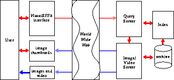
Figure 2: VisualSEEk external system operation.

The VisualSEEk system emphasizes several research goals - automated extraction of localized regions and features, efficient representation of features, preservation of spatial properties, extraction from compressed data [Cha95][CS95] and fast indexing and retrieval. The color indexing component of the system uses the binary color set back-projection algorithm to extract color regions. The user may search for images using both global and local features. For a local color region query the user indicates the locations of the color regions by positioning regions on the query grid (see Figure 3(a)). The returned images can be used for a global query whereby the user selects one image and uses the give me more feature of VisualSEEk to retrieve images that best match the selected one in a specified way (see Figure 3(b)).

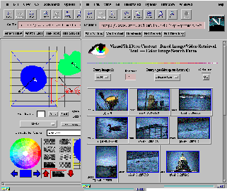
Figure 3: (a) VisualSEEk Java user interface and (b) query returns with give me more feature of VisualSEEk.

Terminology

Thresholding

Thresholding converts a grey level image into a binary image by setting all pixel values above a threshold to 1 and all those below to zero.

Adaptive Thresholding

The process of thresholding with the automatic local selection of a theshold value. Generally this value is estimated from local image content.

Region Growing

An intermediate step in the process of many "image segmentation" algorithms which aims to merge adjacent regions with similar characteristics in order to obtain a simpler and hopefully more correct interpretation of the data.

Image Segmentation

The process of assigning classification groups to an image (often on a pixel by pixel basis) in order to isolate (segment) particular regions of scene structure. Often done as a precursor to higher level interpretation such as recognition or measurement (achieved via the processes of "representation" and "classification").

Split and Merge

A particualr pixel based approach to "image segmentation" whereby the best image segmentation is arrived at by iteratively combining the processes of "region growing" and sub-division.

Histograms

A histogram is an array of non negative integer counts from a set of data, which represents the frequency of occurance of values within a set of non-overlapping regions. For example, the image histogram is an array of the frequency of occurrence of grey levels within a particular set of grey level ranges.

Grey and Binary Scale Levels

A grey level is a single scalar value associated with a particular location in an image. For optical or photographic sensors this value is proportional (or at least monotonically related to) the measured signal. Some sensors or image processing algorithms require multi-valued data such as complex (two valued) or "colour" (three valued) images. Grey level images generally have integer values in the range 0-64, 0-256 or 0-1024, corresponding to 6-bit, 8-bit, or 10-bit digitisation. The binary image requires less storage, one bit per pixel, and is generally used to represent the presence or absence of a particular "feature" at each point in the image (eg: "edges");.

Grey Level Processing

Grey level processing is the general term given to image processing of "grey level" image data. As distict from "binary processing" which refers to processing of binary (single bit per pixel) images.

References

Cha95: S.-F. Chang. Compressed-domain techniques for image/video indexing and manipulation. In I.E.E.E. International Conference on Image Processing, October 1995.
CLP94: T.-S. Chua, S.-K. Lim, and H.-K. Pung. Content-based retrieval of segmented images. In ACM Multimedia 1994, October 1994.
CS95: S.-F. Chang and J. R. Smith. Extracting multi-dimensional signal features for content-based visual query. In SPIE Symposium on Visual Communications and Image Processing, May 1995. Best paper award.
EM95: F. Ennesser and G. Medioni. Finding waldo, or focus of attention using local color information. I.E.E.E. Transactions on Pattern Analysis and Machine Intelligence, 17(8), August 1995.
FFN93: C. Faloutsos, M. Flickner, W. Niblack, D. Petovic, W. Equitz, and R. Barber. Efficient and effective querying by image content. IBM RJ 9453 (83074), August 1993.
HCP95: W. Hsu, T. S. Chua, and H. K. Pung. An integrated color-spatial approach to content-based image retrieval. In ACM Multimedia 1995, November 1995.
HSE95: J. Hafner, H. S. Sawhney, W. Equitz, M. Flickner, and W. Niblack. Efficient color histogram indexing for quadratic form distance functions. I.E.E.E. Transactions on Pattern Analysis and Machine Intelligence (PAMI), July 1995.
Hun89: R. W. G. Hunt. Measuring Color. John Wiley and Sons, 1989.
Jon81: K. S. Jones. Information Retrieval Experiment. Butterworth and Co., 1981.
Rus95: J. C. Russ. The Image Processing Handbook. CRC Press, Boca Raton, 1995.
SB91: M. J. Swain and D. H. Ballard. Color indexing. International Journal of Computer Vision, 7:1 1991.
SC95: J. R. Smith and S.-F. Chang. Single color extraction and image query. In I.E.E.E. International Conference on Image Processing, October 1995.
WS82: G. Wyszecki and W. S. Stiles. Color Science: Concepts and Methods. John Wiley and Sons, 1982.

All of the information about Region Segmentation above is from these links :

Image query

Image can be query from color¡Btexture¡Bshape and layout.On-line collections of images are growing larger and more common, and tools are needed to efficiently manage, organize, and navigate through them. We have developed the QBIC system which lets you make queries of large image databases based on visual image content -- properties such as color percentages, color layout, and textures occurring in the images. Such queries use the visual properties of images, so you can match colors, textures and their positions without describing them in words. Content based queries are often combined with text and keyword predicates to get powerful retrieval methods for image and multimedia databases.

Abstract

In this paper we propose a method for automatic color extraction and indexing to support color queries of image and video databases. This approach identifies the regions within images that contain colors from predetermined color sets. By searching over a large number of color sets, a color index for the database is created in a fashion similar to that for file inversion. This allows very fast indexing of the image collection by color contents of the images. Furthermore, information about the identified regions, such as the color set, size, and location, enables a rich variety of queries that specify both color content and spatial relationships of regions. We present the single color extraction and indexing method and contrast it to other color approaches. We examine single and multiple color extraction and image query on a database of 3000 color images.

Introduction

There is an increasing need for ways to organize and filter the growing collections of image and video data. It is an extremely time consuming task to assign text descriptions to images and the inadequacy of textual annotations for visual data has been recognized. Recently, researchers have begun to investigate "content-based" techniques for indexing images using features such as color, texture and shape [1][2]. A successful content-based image database system requires the following components:

* identification and utilization of intuitive visual features

* effective feature representation and discrimination

* automatic extraction of spatially localized features

* techniques for efficient indexing

In this paper we investigate the use of color for organizing and retrieving images and videos from databases. We maintain that color is an intuitive feature for which it is possible to utilize an effective and compact representation. Our approach automatically extracts the color content of isolated regions within images and builds efficient indexes to retrieve the regions over a large collection of images. The spatial localization of the color regions also allows for queries to include spatial positions and relationships between color regions. This gives a great power of expression for database queries that include both specification of color sets and relative and absolute spatial locations.

Queries supported by the single color technique include the following examples: give me all images containing...

a.) a large dark green area near top of image, i.e., trees

b.) a yellowish-orange spot surrounded by blue, i.e., a sunset

c.) a region composed of red, white and blue, i.e., a flag

d.) an area with red and white in equal amounts, i.e., a checkered table cloth.

We will explain how these queries can be answered using color sets with one or more colors, and/or by specifying spatial relationships and composition of regions.

Color Features

Color may be one of the most straight-forward features utilized by humans for visual recognition and discrimination. However, people show the natural ability of using different levels of color specificity in different contexts. For example, people would typically describe an apple as being `red', probably implying some type of reddish hue. But in the context of describing the color of a car a person may choose to be more specific instead using the terms `dark red' or `maroon'. Color extraction by computer is performed without benefit of a context. Lack of knowledge also makes it difficult to cull the color information from the color distortion. The appearance of the color of real world objects is generally altered by surface texture, lighting and shading effects, and viewing conditions. Image database systems that use color retrieval must grapple with these problems of automated color image analysis.

Color histogram

One common method for characterizing image content is to use color histograms. The color histogram for an image is constructed by counting the number of pixels of each color. Retrieval from image databases using color histograms has been investigated in [1][2][3]. In these studies the formulations of the retrieval algorithms follow a similar progression: (1) selection of a color space, (2) quantization of the color space, (3) computation of histograms, (4) derivation of the histogram distance function, (5) identification of indexing shortcuts. Each of these steps may be crucial towards developing a successful algorithm. But there has been no consensus about what are the best choices for these parameters. In [1] we evaluated the retrieval performance when several of these parameters were varied on a database of 500 color images.

There are several difficulties with histogram based retrieval. The first of these is the high dimensionality of the color histograms. Even with drastic quantization of the color space, image histogram feature spaces can occupy over 100 dimensions in real valued space. This high dimensionality ensures that methods of feature reduction, pre-filtering and hierarchical indexing must be implemented. The large dimensionality also increases the complexity and computation of the distance function. It particularly complicates `cross' distance functions that include the perceptual distance between histogram bins. Another challenge with the use of color histograms is to enable the extraction of localized features.

Color image segmentation

The extraction of spatially localized features is an extremely important aspect of image indexing. The isolated regions of interest within images should be identified and extracted independently from other regions in the image. For example, an image should be retrieved even when the user can describe only part of the image. If each image is represented by a single color histogram, this aspect of retrieval performance declines significantly. This is because extraneous information such as background colors may dominate the histogram.

Several attempts have been made to improve performance. In [1] images were segmented into fixed blocks and each block was indexed separately. In this way some blocks may still retain a reasonable characterization of objects of interest. On the other hand, the QBIC system [2] requires manual segmentation of images. In QBIC the color histograms are computed as attributes of the regions that have been cut out by hand. This reduces the potential contribution of background and other irrelevant colors but requires extensive human involvement in creation of the indexed data. Automated segmentation of images using color histograms may eventually provide useful results but has not yet been integrated into large image retrieval systems.

Single Color extraction

The goal of the single color extraction method is to reduce the dimensionality of the color feature space while gaining the ability to localize color information spatially within images. Illustrated in Figure 1, we accomplish this through the following means: reduction of the full gamut of colors to a set of manageable size (~100 carefully selected colors). We avoid mapping unacceptably dissimilar colors into the same bins. We also allow higher tolerance in color lightness and color saturation while reserving the most fine quantization for hue. We utilize a `colorizing' algorithm to paint the color images using the reduced palette and a broad brush. This ensures that the most dominant colors and regions are emphasized. The processed images retain a visibly acceptable and compact representation of the color content. After this processing, we search over the set of colors remaining in the image, and map the regions that sufficiently contain the selected colors into a database index. The next section discusses the process in more detail.

Color space

The RGB color format is the most common color format for digital images. The primary reason for this is because it retains compatibility with computer displays. However, the RGB space has the major drawback in that it is not perceptually uniform. Because of this, uniform quantization of RGB space gives perceptually redundant bins and perceptual holes in the color space. Furthermore, ordinary distance functions defined in RGB space will be unsatisfactory because perceptual distance is a function of position in RGB space.

Other color spaces, such as CIE-LAB, CIE-LUV and Munsell offer improved perceptual uniformity [4]. In general they represent with equal emphasis the three color variants that characterize color: hue, lightness, and saturation. This separation is attractive because color image processing performed independently on the color channels does not introduce false colors [5]. Furthermore, it is easier to compensate for many artifacts and color distortions. For example, lighting and shading artifacts will typically be isolated to the lightness channel. In general, these color spaces are often inconvenient due to the basic non-linearity in forward and reverse transformations with RGB space. For color extraction we utilize the more tractable HSV color space because it has the above mentioned characteristics and the transformation from RGB space is non-linear but easily invertible.

The next issue after color space selection is quantization. The HSV color space can be visualized as a cone. The long axis represents value: blackness to whiteness. Distance from the axis represents saturation: amount of color present. The angle around the axis is the hue: tint or tone. Quantization of hue requires the most attention. The hue circle consists of the primaries red, green and blue separated by 120 degrees. A circular quantization at 20 degree steps sufficiently separates the hues such that the three primaries and yellow, magenta and cyan are represented each with three sub-divisions. Saturation and value are each quantized to three levels yielding greater perceptual tolerance along these dimensions. The quantized HSV space appears in Figure 3.

Color processing

To identify color regions, the images are transformed to the quantized HSV space with 166 color bins and subsampled to approximately 196x196 such that correct aspect ratio is preserved. This generally reduces the image content to less than 50 colors. Even after the transformation it is still premature to isolate color regions because small details and spot noises interfere. We reduce most of this insignificant detail by using a colorizing algorithm. This processing is accomplished using a 5x5 median filter on each of the HSV channels. This non-linear filtering in HSV space does not introduce false hues. The color image is then converted back to an indexed RGB space. Table 1 reports the statistics of color processing of 3000 color images.

Color region labelling

The next step involves the extraction of the color regions from the images. This is done by systematically selecting from the colors present in the image one at a time, and in multiples, each time generating a bi-level image. The levels correspond to the selected and un-selected pixels for the specified color set. Refer to Figure 2 and Table 2 for an illustration of region extraction and representation of the Butterfly color image. Next follows a sequential labelling algorithm that identifies the isolated regions within the image. The characteristics of each color region are evaluated in regards to several thresholds to determine whether the region will be added to the database. The first threshold is one for region size. In our system the region must contain more than 64 pels to be significant. This value still allows for sufficiently small regions to be indexed.

If more than one color is represented in the color set we utilize two additional thresholds. The first threshold is the absolute contribution of each color. If a color does not contribute at least 64 pels to the region, the region is not added. Furthermore, the relative contribution is also measured. All colors must contribute to at least 20% of the region area. Notice that this produces a firm limit of 5 colors per color region although, we use only up to 3 colors at a time. If a color region does not pass one of these thresholds then it will not be indexed by that color set. If a region is rejected because one of the colors from the color set is not sufficiently represented, the region still has a chance to be extracted using a reduced color set leaving out the under-represented color. Enforcing the color set thresholds prevents the unnecessary and redundant proliferation of indexed multiple-color regions.

Color image mining

Even with the reasonably small color gamut it is necessary to search systematically for multiple color regions. Otherwise, it will require 2m passes over the image to test all combinations of m colors. We utilize a heuristic similar to that used for database mining [6]. The algorithm makes multiple passes over each image, expanding only the color sets that meet minimum support constraints. A color set Ci of binary colors is explored for an image only if for all colors k in Ci, where Ci[k]=1, there are at least t0 pixels in the image of color k such that t1 pixels of color k have not yet been allocated to a color region. We use t0 and t1 = 64. If t0 is not met then Ci will have colors that cannot be represented sufficiently by any color regions. Exploring this color set and all supersets of it would be futile. If t0 is met while t1 is not, then a color region containing all of the colors in Ci can alternatively be reconstructed using subsets of Ci and spatial composition. Therefore, exploration of Ci and its supersets generate redundant information.

Figure 4 illustrates an example of the extraction of an American flag in the San Francisco color image. The region was extracted in whole while searching over color sets in the extraction process. The region and color set met the constraints to allow the region to be extracted. The users request for a {red, white, blue} region is answered with the minimum bounding rectangle in Figure 4(d) that represents the region.

Color specification and spatial positions

The color characteristics specified by the user are represented using the m-dimensional binary color vector. The values may be obtained by picking colors from a color chooser, by navigating visually through 3-D color space, or by textual specification. The binary color vector will be quickly matched to region data because we allow only up to three colors per color set for each indexed region. This sparse binary vector representation of the color sets makes it far easier to index the color distributions than that needed for the color histogram techniques.

After the color characteristics of the regions have been determined, the spatial positions and relationships between regions can be specified by the user. The spatial characteristics of the color region query can be handled using one of several techniques that have been devised for representing and querying spatial information [7][8].

Conclusions and future work

Single color query is an extremely useful content-based query tool for users of image and video databases. We proposed a method for automatically extracting the single and multiple color regions within images. The color extraction approach allows interesting queries to be formulated based on size, shape and spatial relations of the color regions. The single color approach allows the user to specify the color content and spatial positions of region within images. Single color extraction and indexing is supported in the Content-Based Visual Query System being developed at Columbia University for a variety of image and video applications.

References

[1.] John R. Smith and Shih-Fu Chang, "Tools and Techniques for Color Image Retrieval," submitted to ACM Multimedia 95.

[2.] C. Faloutsos, et. al., "Efficient and Effective Querying by Image Content," IBM RJ 9453 (83074), August 3, 1993.

[3.] M. Swain and D. Ballard, "Color Indexing," International Journal of Computer Vision, 7:1, 1991, p. 11 -- 32.

[4.] G. Wyszecki and W. S. Stiles, Color Science: Concepts and Methods, John Wiley & Sons, 1982.

[5.] John C. Russ, The Image Processing Handbook, IEEE Press, 1995.

[6.] R. Agrawal, et. al, "Mining Association Rules between Sets of Items in Large Database," ACM SIGMOD-93, Washington, DC, May, 1993.

[7.] T. Gevers and A.W.M. Smeulders, "An Approach to Image Retrieval for Image Databases," Database and Expert System Applications (DEXA-93), 1993.

[8.] S. K. Chang, et. al., "An Intelligent Image Database System," I.E.E.E. Transactions on Software Engineering, Vol. 14, No. 5, May 1988.

[9.]http://wwwqbic.almaden.ibm.com/

[10.]http://www.ctr.columbia.edu/~jrsmith/html/pubs/ICIP-95-2/single1.html

To appear at the International Conference on Image Processing (ICIP-95), Washington, DC, Oct. 1995

FIGURE 1. Car color Image: (1) conversion to HVS color space, (2) quantization of HVS space, (3) color median filtering, (4) conversion to indexed RGB space, (5) the processed color image has dominant color regions emphasized.

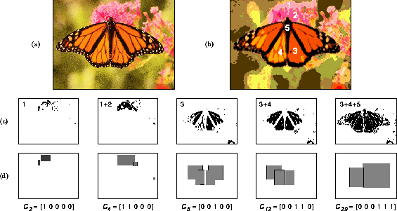
FIGURE 2. (a) Butterfly color image, (b) processed color image with 30 colors, (c) pixels from image (b) belonging to color set Ci, (d) minimum bounding rectangles (MBRs) for extracted regions used to index the image collection.

FIGURE 3. Quantized HSV color space, 18 hues, 3 saturations and 3 values + 4 grays = 166 colors.

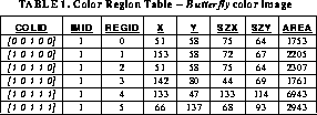
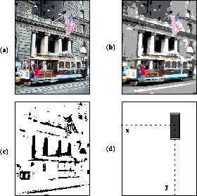
FIGURE 4. (a) San Francisco color image, (b) processed image with 73 colors, (c) pixels belonging to color set = {red, white, blue}, (d) extracted color region as present in index.

A Color Segmentation Algorithm to Annotate Fine Art Images

演講摘要

目的：

動機：

前人的研究：

OUTLINE：

結論：

FUTURE WORK：

演講詳細內容：

Introduction

Colorspace

1.what is colorspace

2.RGB

3.CMYK

4.Relation

Region Segmentation

General Approach

Region Extraction/Segmentation

Region Feature Extraction

Color Image Retrieval Systems

VisualSEEk

Terminology

References

Image query

Abstract

Introduction

Color Features

Color histogram

Color image segmentation

Single Color extraction

Color space

Color processing

Color region labelling

Color image mining

Color specification and spatial positions

Conclusions and future work

References

相關網站